Convective Rolls in a Compressible Fluid

Katherine J. Simzer
Department of Atmospheric and Oceanic Sciences, McGill University, Montreal, QC, Canada

Gregory M. Lewis
Faculty of Science, University of Ontario Institute of Technology, Oshawa, ON, Canada

Abstract

Introduction

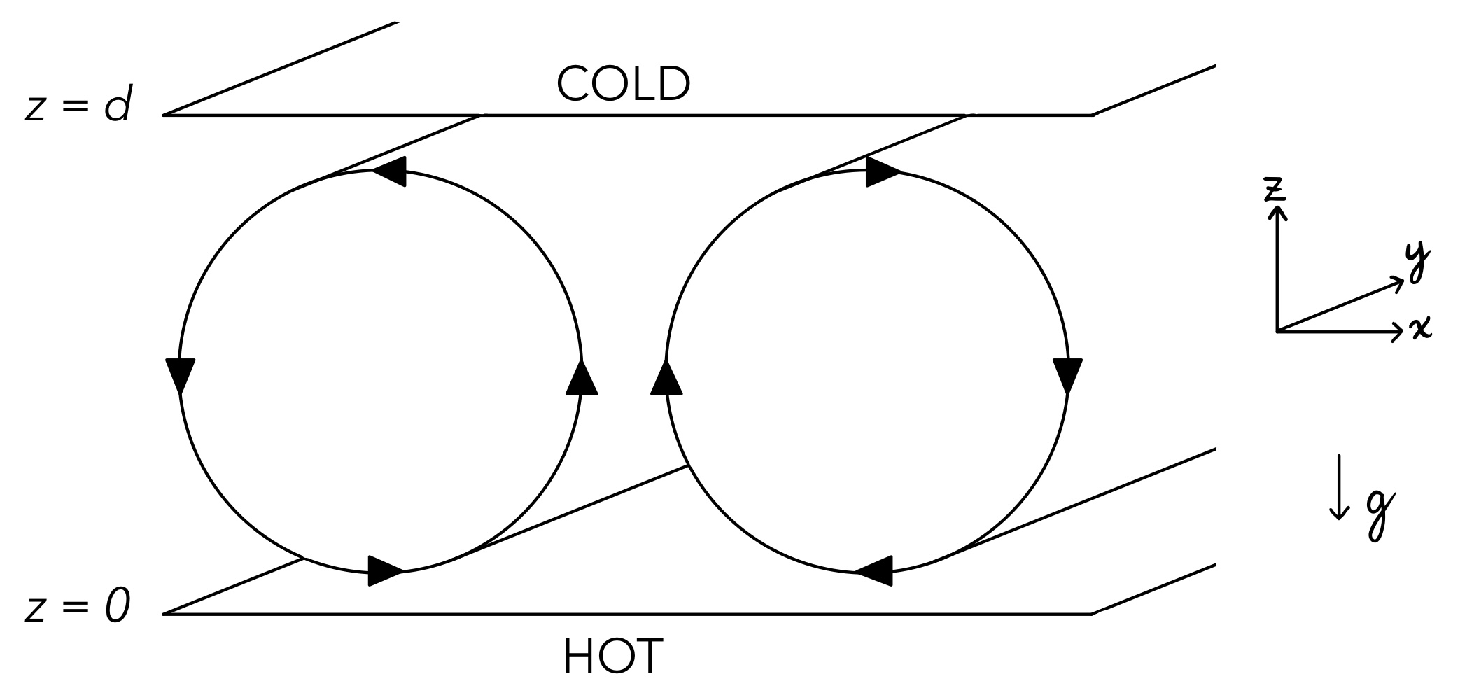
Rayleigh-Bénard convection occurs in a fluid confined between two horizontally infinite plates when the lower plate is heated with respect to the upper one. When the temperature difference between the two plates is sufficiently large, the fluid begins to flow, as the warmer fluid below becomes more buoyant than the cooler fluid above it. This problem was first studied by Lord Rayleigh, in the context of an approximately incompressible fluid. (1,2) The onset of convection leads to the formation of patterns in the fluid. As the temperature difference between the plates is increased further past the critical value required to support fluid flow, the pattern seen in the fluid becomes increasingly more complicated. (3-5) This paper will consider the simplest pattern that is known to occur near the onset of convection, which consists of straight, parallel convection rolls; (5,6) see Fig. 1. This work is inspired by convection in the atmosphere, and, thus, will investigate the onset of these rolls in a compressible, vertically-stratified fluid which we model using the anelastic equations, which have been used extensively to model convection in the atmosphere. (7,8) Natural convective patterns in the atmosphere tend to vary greatly in time and across the horizontal plane, but they do keep a similar vertical structure to these idealized convective rolls. (5)

The standard classical analysis of Rayleigh-Bénard convection uses the Boussinesq approximation, (9) in which variations in the density of the fluid are only accounted for in the buoyancy term, and thus the fluid is considered to be incompressible. This approximation requires low Mach-number and neglects acoustic frequencies. Work has been done to study the validity of the Boussinesq approximation in a compressible fluid in the context of the onset of convection, (10) which shows that it is only valid when the vertical dimension of the fluid is much less than any scale height. This implies that, in this context, the Boussinesq approximation will not hold at the spatial scales of the atmosphere.

Jeffreys (1930) found that instability in a compressible fluid arises only once the temperature gradient exceeds the adiabatic one. (11) They propose that the excess temperature gradient could be found by the same formula which gives the gradient needed for instability in a Boussinesq fluid. However, they conclude that this can only be applied directly when density does not vary greatly in the system. Spiegel (1965) verified Jeffreys’ claim by performing a perturbation expansion in terms of layer thickness. (12) Non-Boussinesq convection with no-slip top and bottom boundaries has been studied by Tilgner (2011), using parameter values fitting the terrestrial troposphere. (13) They conclude that data collapse is obtained when an effective density given by the geometric mean of the maximum and minimum densities in the convecting layer is introduced to the scaling laws.

Other studies have looked at the anelastic approximation for a compressible fluid. This approximation was first proposed by Ogura and Charney (1960), (14) who implemented the anelastic approximation by filtering out the sound waves from the adiabatic motions of an inviscid fluid. (15) Further analysis of anelastic convection by a one-parameter expansion was done by Gough (1969), showing that molecular and radiative transport processes are approximately static on a convective timescale in the atmosphere. (15) In both papers, the range of the temperature is assumed to be close to the minimum required to produce the onset of convection. In the context of stellar convection, Spiegel (1965) studied the onset of convection in a polytropic atmosphere using a perturbation expansion in terms of layer thickness. (12)

There have been further studies of non-Boussinesq fluids in a variety of other contexts as well. Burnishev, Segre, and Steinberg (2010) looked at heat transport in turbulent convection of SF₆ near its gas-liquid critical point, and found that there is a symmetrical vertical dependence of the main physical properties such that the temperature in the midplane of the cell stays equal to the average value, despite the variations in fluid properties across the cell height. (16) Ahlers et al. (2007) experimentally measured and then calculated the non-Boussinesq effects of strongly turbulent convection in ethane gas, finding a decrease of the central temperature compared to the mean of the top- and bottom-plate temperatures in the Boussinesq case. For the case of a numerical simulation of a perfect gas contained in a rigid box, Robinson and Chan (2004) found that a strong enough stratification caused changes in the observed bifurcation, where the signs of the thermal perturbations became antisymmetric about the roll center instead of symmetric as seen without the stratification. (17)

This paper will present an analysis of the onset of convection in a compressible fluid and compare the results with those for a fluid that follows the Boussinesq approximation shown in, for example, Acheson (1990) (18) and Kundu and Cohen (2002). (19) In this context, we seek a quantitative measure for the spatial scale at which the Boussinesq approximation breaks down for the parameter values relevant to the Earth’s atmosphere, and we seek to determine how this value changes when the viscosity of the fluid is changed.

Model

We consider the problem of the onset of motion in a layer of fluid contained between two infinite horizontal plates, where the plates are sepa rated by a distance d, the lower plate is held at a temperature T₁, and the upper plate is held at T₁ − ΔT. We model the flow of the fluid with the 3-D Navier-Stokes equations together with the thermodynamic energy equation for dry air and the mass continuity equation. (20) We assume that the equation of state of the fluid is given by the ideal gas law. In an isothermal atmosphere in hydrostatic balance, the hydrostatic pressure p₀ and density ρ₀ vary only with height z and are given explicitly by

where H = R_*T₀/g is a scale height, R_* is the ideal gas constant, g is the gravitational constant, T₀ is a constant reference temperature defined as p₀/(R_*ρ₀), and p₀₀ = p₀(z = 0) and ρ₀₀ = ρ₀(z = 0) are a reference pressure and density, respectively. We make the assumption that the density and pressure exhibit only small deviations from these profiles, which is a reasonable approximation for the atmosphere. (20) In particular, elastic variations in the flow, such as sound waves, are filtered. The resulting equations are generally referred to as the anelastic equations. We therefore write the pressure p = p₀+p', density ρ = ρ₀+ρ', and absolute temperature T = T₀+T' of the fluid, where

\[ \left| \frac{p^\prime}{p_0} \right| < < 1, \qquad \left| \frac{\rho^\prime}{\rho_0} \right| < < 1, \qquad \left| \frac{T^\prime}{T_0} \right| < < 1. \]

In addition, we make the assumption that the deviations from the static vertical profile satisfy

\[ \left| \frac{\rho^\prime}{\rho_0} \right| \approx - \left| \frac{T^\prime}{T_0} \right|, \]

which is expected to be a good approximation when the distance d between the plates is small relative to the scale height H. With these approximations, we can eliminate the density deviation ρ′, and the momentum equation becomes

\begin{equation} \rho_0 \frac{D \vec{u}}{Dt} = -2 \rho_0 \vec{\Omega} \times \vec{u} - \nabla p^\prime - \frac{\rho_0}{T_0} \vec{g} T^\prime + \mu \nabla^2 \vec{u}, \label{eq:mom} \end{equation}

the thermodynamic equation becomes

\begin{equation} \rho_0 c_V \frac{D T^\prime}{Dt} = -\rho_0 g w + k \nabla^2 T^\prime + Q, \label{eq:thermo} \end{equation}

and the continuity equation becomes

\begin{equation} \nabla \cdot (\rho_0 \vec{u}) = \nabla \cdot\vec{u} - \frac{w}{H}= 0, \label{eq:cont} \end{equation} where $\vec{u} = (u,v,w)$ is the fluid velocity vector in a Cartesian coordinate system $(x,y,z)$ rotating at rate $\vec{\Omega}$, $\vec{g}= -g$, \[ \frac{D}{Dt} = \frac{\partial}{\partial t} + \vec{u} \cdot \nabla, \qquad \nabla = \hat{x} \frac{\partial}{\partial x} + \hat{y} \frac{\partial}{\partial y} + \hat{z} \frac{\partial}{\partial z}, \] the Laplacian $\nabla^2 = \nabla \cdot \nabla$, $\mu$ is the dynamic viscosity or alternatively an Eddy viscosity coefficient, $k$ is the thermal conductivity, $c_V$ is the specific heat at constant volume, and $Q$ is the heating rate due to, for example, radiant and latent heat. We have assumed that the dynamic viscosity $\mu$ and the thermal conductivity $k$ are constant.

For the boundary conditions, we assume no-slip at both plates. That is, the fluid will have zero velocity relative to the boundary. The temperature at the upper and lower plate is fixed at the prescribed values.

Equations \eqref{eq:mom} -- \eqref{eq:cont} define a closed system for the fluid velocity $\vec{u}$, temperature deviation $T^\prime$, and pressure deviation $p^\prime$. Similar equations appear in Spiegel (1965), (12) except that \eqref{eq:mom} -- \eqref{eq:cont} use a simpler form of the viscosity and relation between the temperature and density deviations. We follow Spiegel (1965) and choose to work with the equations in dimensional form, because non-dimensionalization does not simplify the analysis. (12) In particular, in this context, the Rayleigh number depends on height $z$. However, to facilitate comparison with the classical results, we will present our results in terms of the Rayleigh number ${\cal R}_h$ at the centre height between the plates \begin{equation} {\cal R}_h = \frac{g c_p \left( \frac{\Delta T}{d} - \frac{g}{c_p} \right) d^4 \rho_{00}^2}{T_0 k \mu} e^{-d/H}, \label{eq:Rayleigh_halfheight} \end{equation} as in Spiegel (1965), where $c_p$ is the specific heat at constant pressure. (12) This is similar to the standard definition of the Rayleigh number except that it includes the vertical variation in the basic density profile, and the difference $\Delta T/d - g/c_p$ of the imposed temperature gradient and the adiabatic lapse rate replaces the temperature gradient alone. The latter emphasizes that the imposed temperature gradient must overcome the adiabatic lapse rate before instability can set in.

In this paper, we consider a non-rotating system and we assume that there is no source of heating other than the plates. That is, we take $\vec{\Omega} = 0$ and $Q=0$. The effects of these choices on the dynamics will be considered in subsequent investigations.

Analysis

In the absence of motion, an analytical solution can be found in which the temperature has a linear dependence on $z$, where $z$ has bounds from $z=0$ to $z=d$. This solution is the conduction solution $T^\prime = T_{cd}$, where \[ T_{cd} = \Delta T \left( \frac{-z}{d} + \frac{1}{2} \right), \] and we have chosen $T_l = T_0 + \Delta T/2$. It is convenient to write $T^\prime = T^{\prime\prime} + T_{cd}$, in which case the thermodynamic equation becomes \begin{equation} \rho_0 c_V \frac{D T^{\prime\prime}}{Dt} = -\rho_0 \left(g - \frac{c_V \Delta T}{d} \right) w + k \nabla^2 T^{\prime\prime}, \label{eq:thermo_pert} \end{equation} with corresponding boundary conditions $T^{\prime\prime}(z=0) = T^{\prime\prime} (z=d) = 0$. Written as such, $T^{\prime\prime}=0$, $w=0$ is the solution of \eqref{eq:thermo_pert}, which corresponds to the conduction solution.

For sufficiently low values of $\Delta T$, the conduction solution is stable. We expect the onset of convection to occur at the value of $\Delta T$ for which the conduction solution becomes unstable to some small perturbation. In particular, we seek the parameter value $\Delta T = \Delta T_c$ for which perturbations decay for $\Delta T < \Delta T_c$, and for which at least one form of perturbation grows for $\Delta T > \Delta T_c$. Because we consider only small perturbations, we can determine their dynamics from the linearization about the conduction solution.

We will restrict our attention to the case where the solutions at onset correspond to convective rolls (see Fig. 1), where the flow consists of spatially periodic pairs of counter-rotating cylindrical cells. As such, we consider only perturbations of this form. In this case, by orienting the $y$-axis along the lengthwise direction of the rolls, we can assume that $v=0$ and that the solutions do not depend on $y$. We can therefore use a modified stream function, $\psi$, which ensures the continuity equation \eqref{eq:cont} is implicitly satisfied. In particular, we choose $\psi = \psi(x,z,t)$ such that \begin{equation} u = \frac{1}{\rho_0} \frac{\partial \psi}{\partial z}, \qquad w = -\frac{1}{\rho_0} \frac{\partial \psi}{\partial x}. \label{eq:stream_fn_defn} \end{equation} If we take the curl of the linearized momentum equation \eqref{eq:mom}, we can eliminate the pressure, and obtain \begin{equation} \frac{\partial}{\partial t} \left( \nabla \times \rho_0 \vec{u} \right) = -\frac{\rho_0}{T_0} \nabla T^{\prime\prime} \times \vec{g} + \mu \nabla^2 (\nabla \times \vec{u}). \label{eq:curl} \end{equation} We can determine the evolution of $\psi$ from the $y$-component of \eqref{eq:curl} \begin{equation} \frac{\partial}{\partial t} \nabla^2 \psi = -\frac{\rho_0 g}{T_0} \frac{\partial T^{\prime\prime}}{\partial x} + \mu \nabla^2 \left( \frac{1}{H \rho_0} \frac{\partial \psi}{\partial z} + \frac{1}{\rho_0}\nabla^2 \psi \right), \label{eq:streamfn_eqn} \end{equation} where we have eliminated $u$ and $w$ using \eqref{eq:stream_fn_defn}. This equation together with the linearization of \eqref{eq:thermo_pert} defines a closed system that describes the evolution of the perturbations $\psi$, $T^{\prime\prime}$ when these are small. The corresponding boundary conditions are \[ \psi=0, \quad \frac{\partial \psi}{\partial z} = 0, \quad T^{\prime\prime} = 0, \quad {\rm at} \ \ z=0,d. \] The second boundary condition on $\psi$ ensures that the horizontal velocity $u$ vanishes on the boundaries. In order to ensure that the vertical velocity $w$ vanishes, we only require that $\psi$ is constant on the boundaries. If this constant were different on the top and bottom boundaries, then there would be a net (average) flow in the $x$-direction, which is not expected due to the symmetry of the problem. We can, therefore, take $\psi=0$ on both boundaries, because $\psi$ is only determined up to an additive constant. Because the convective rolls are spatially-periodic in the horizontal for some unknown period, we seek separable solutions of the form \begin{equation} \psi=e^{\lambda t}\hat{\psi} (z)e^{iax}, \qquad T^{\prime\prime}=e^{\lambda t}\hat{T}(z)e^{ iax}, \label{eq:soln_form} \end{equation} where $2\pi/a$ is the horizontal spatial wavelength of the solution and, therefore, $\pi/a$ gives the horizontal extent of each roll. Substitution of \eqref{eq:soln_form} into the linearized equations results in a (generalized) linear differential eigenvalue problem for the eigenvalues $\lambda$ \begin{equation} \lambda A U = L U, \label{eq:eig_prob} \end{equation} where $A$ and $L$ are linear ordinary differential operators and $U=U(z) = [\hat{\psi}, \hat{T}]$. In particular, the operators $A$ and $L$ involve up to fourth-order derivatives with respect to $z$; they will also depend on $a$ and $\Delta T$. If for a given $\Delta T$, all eigenvalues corresponding to all $a$ have a negative real part, all small perturbations of the form \eqref{eq:soln_form} will decay, and the conduction solution will be asymptotically stable. If any eigenvalue corresponding to any value of $a$ has positive real part, the associated perturbations will grow, and the conduction solution is unstable. Therefore, if, for each $a$, we find the $\Delta T$ at which a single eigenvalue has zero real part, while all other eigenvalues have negative real part, then onset of convection will occur at the minimum such value of $\Delta T$. That is, at the critical temperature difference $\Delta T_c$ a single eigenvalue for $a=a_c$ will have zero real part and all other eigenvalues associated with all other values of $a$ will have negative real part. This process is not able to determine the full form of the solution for $\Delta T > \Delta T_c$ because it is not able to determine the possible variations that may occur in the $y$-direction. In particular, in the classical Rayleigh-B\'enard convection, close to onset, both rolls and hexagonal cells can be observed \citep{Acheson}. Thus, it is expected that our analysis will only determine the critical $\Delta T_c$ and the preferred horizontal spatial scale $a=a_c$ of the solution. The eigenvalue problem \eqref{eq:eig_prob} cannot be solved analytically, and therefore we use second-order centred finite differences to discretize in the $z$ direction on a uniform grid. Upon discretization, the problem is reduced to a matrix eigenvalue problem. The solution process is implemented in Python using LAPACK subroutines from the SciPy linear algebra module, which is expected to be accurate to round-off error. For all calculations, we discretize the vertical using $N=100$ uniformly-spaced grid points; some of the computations are verified by also using $N=50$ and $N=200$ grid points. Table 1 lists the values of the parameters used in the solution.

Table 1. Values of paramaters used

Variable	Value
g	9.81 [m s-1]
cv	716 [J kg-1 K-1]
k	0.0227 [W m-1 K-1]
ρ0	1.412 [kg m-3]
H	7310 [m]
T0	250 [K]
R*	287.058 [J kg-3 K-3]

Results

For each value of the plate separation distance $d$ that we consider, we seek the minimum value of the temperature difference $\Delta T$ for which the conduction state is neutrally stable. That is, we seek the critical temperature difference $\Delta T_c$ for which a single eigenvalue associated with wave number $a=a_c$ has zero real part while all other eigenvalues associated with all other values of $a$ have negative real part. The eigenvalues are determined from Eq. \ref{eq:eig_prob}, from which the evolution of perturbations from the conduction solution of the form \eqref{eq:soln_form}, can be determined. If we increment through a range of values of the wave number $a$, and for each $a$, we find the critical temperature difference associated with that specific wave number, then $\Delta T_c$ and $a_c$ can be found where this critical temperature difference as a function of the wave number $a$ achieves its minimum. Fig. 2 is an example of a plot of the Rayleigh number at half-height (see Eq. \ref{eq:Rayleigh_halfheight}) calculated using the critical temperature difference as a function of wave number for plate separation $d = 0.1$m, for which ${\cal R}_h = 2390.77$ and $a_c=31$m$^{-1}$. In this case, and in all others that we consider, it is found that the critical eigenvalue is real, i.e. it is equal to zero.

The overall minimum critical temperature difference $\Delta T_c$ and its corresponding value of $a_c$ are calculated for different plate separation distances $d$, with the corresponding Rayleigh number calculated at the half-height. Fig. 3a highlights the relationship between $d$ and ${\cal R}_h$; for these calculations, the dynamic viscosity $\mu=15.98 \times 10^{-3}$kg m$^{-1}$ s$^{-1}$, and values for the other parameters are listed in Table 1. Two different trends can be seen, with lines of best fit that intersect where $d=1.28$m. Spiegel (1965) found that in the limit of very small layer thickness the problem of convective stability is exactly represented by the Boussinesq equations as modified by Jeffreys (1930). (11, 12) This is what we see for values of $d$ less than $1.28$m, where the Rayleigh number at the half-height for the onset of convection is approximately constant with $d$. For values of $d$ greater than $1.28$m, the Rayleigh number at half-height increases for increasing $d$. Specifically, the slope of the line of best fit on the log-log plot for $d>1.28$m is 3.97, which implies the approximate relation ${\cal R}_h \propto d^4$. The extra data points around the point of intersection of the two lines of best fit in Fig. 3a allow us to see that the transition between the two relationships is smooth.

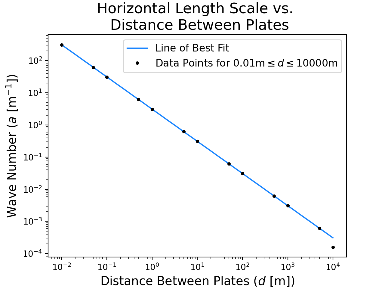
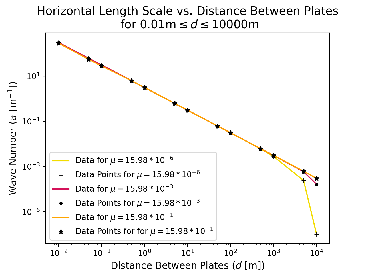
Fig. 3b shows the relationship between the wave number $a$ and the plate separation distance $d$. Except for the largest value of $d$, this relationship is linear with slope -1.00 and intercept 3.10 on this log-log plot, implying that $a_c \approx 3.1/d$, approximately. The points where $d=5000$m and $d=10000$m do not fit well to the line of best fit, with corresponding values of $a$ being smaller than expected; we have not included these points in the best fit calculation.

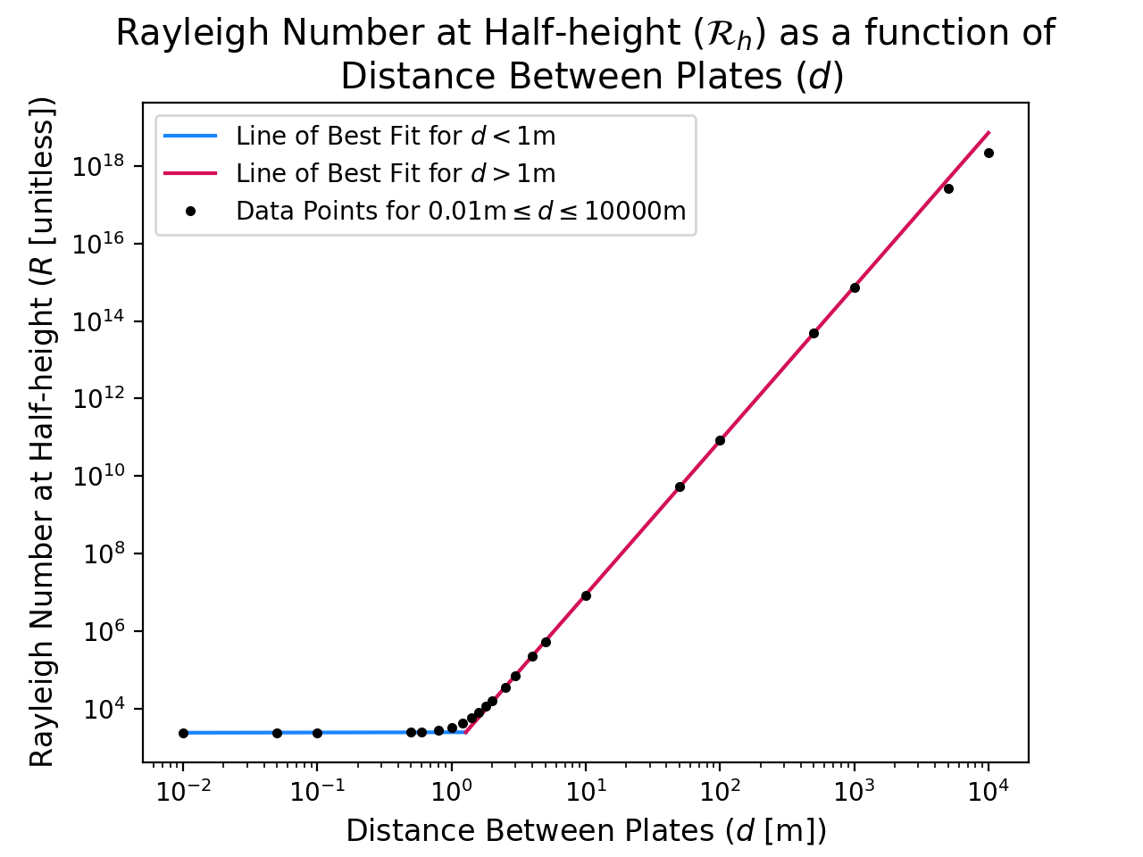
In the classical case addressed by Rayleigh (1916) (see Acheson (1990)), where it is assumed that the fluid is modelled well by the Boussinesq approximation and stress-free boundary conditions are used, (1, 18) the relationship between the critical wave number $a_c$ and plate separation distance $d$ is given by the expression \begin{equation} a_c = \frac{\pi}{\sqrt{2} d}. \label{eq:a_d} \end{equation} with corresponding critical Rayleigh number given by \begin{equation} {\cal R}_c = \frac{ \alpha g c_p \rho_0^2 \Delta T_c d^3}{\mu k} = \frac{27 \pi^4}{4} \end{equation} where $\alpha$ is the coefficient of thermal expansion, and $\rho_0$ is constant. When more realistic boundary conditions are employed, the corresponding critical values are $a_c \approx 3.1/d$ and ${\cal R}_c \approx 1708$ (see Kundu and Cohen (2002)). (19) We employ the more realistic boundary conditions, and therefore we expect our results to compare more closely to these. In these classical problems, the critical Rayleigh number is independent of plate separation distance $d$. However, it is clear from Fig. 3a that this is not the case for a compressible fluid. At small $d$, the critical Rayleigh number at half-height is approximately constant with $d$. However, for $d > 1$m, the critical Rayleigh number at half-height grows with $d$; in particular, there is a ${\cal R}_h \propto d^4$ relationship. The Rayleigh number at half-height approaches the standard Rayleigh number when $d$ is small, and therefore it may be expected that the critical value for small $d$ in the compressible case should approach that of the classical case. However, even in the limit as $d$ goes to zero, the Boussinesq equations are only completely recovered from our anelastic equations when $c_p$ is replaced with $c_v$ (see Spiegel and Veronis). (10) If we do this, we recover the classical ${\cal R}_c = 1708$ result for the smallest values of $d$, as expected, which provides some validation for our numerical results, as well. Although a discrepancy is observed in the critical Rayleigh number at half-height, the relationship between the critical wave number $a_c$ and plate separation distance $d$ for the compressible and Boussinesq cases only differ at the largest $d$. In particular, both cases exhibit an $a_c \approx 3.1/d$ relationship, except for the two largest values of plate separation distances where $d=5000$m and $d=10000$m, at which the compressible case deviates.

These results have been verified by repeating the calculations with $N=50$ and $N=200$ grid points. Most values of $\Delta T_c$ have a percentage change much less than 1%, with only $d=0.01$m having a larger change for $N=200$. For values of $a$, most have no change with the exception of the largest $d$ for $d = 5000$m and $d = 10000$m. This could explain the deviations in the results for large $d$ in the graph of $a$ vs. $d$. The reason for this is likely because at the small scales of $a$ when $d$ is large, there are only very small changes in ${\cal R}_h$ when trying to obtain the minimum, so the error in finding the true minimum $a_c$ is higher.

Effects of Viscosity

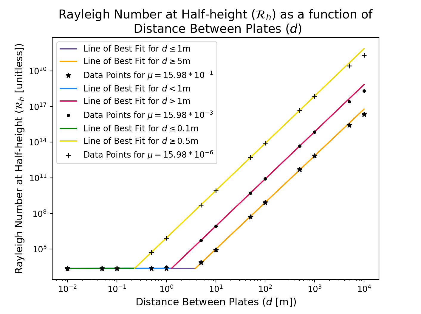
The plots shown in Fig. 3 are recreated for a larger and smaller value of the dynamic viscosity $\mu$. The viscosities we use differ greatly from the viscosity of dry air at atmospheric pressure since $\mu$ can alternatively be interpreted as an eddy viscosity coefficient. The value of the eddy viscosity coefficient depends on the flow rather than the physical properties of the fluid (Holton, 2004), (20) so changes in the eddy viscosity may reflect changes in the smaller scale fluctuations within the fluid. As previously, the values for all the other parameters are taken to be those listed in Table 1; see Fig. 4 and Fig. 5. All of the plots have the same general trends, except with significant differences in the points of intersection of the lines of best fit, which are listed in Table 1. These points of intersection signify where compressible and Boussinesq fluids begin to differ, where the value of ${\cal R}_h$ begins to increase significantly. The data shows that the higher the viscosity of the fluid is, the larger the value of $d$ and the smaller the value of $a$ will be for the Rayleigh number to start increasing, and vice versa. The plots for each value of viscosity can be seen together in Fig. 4. Despite the differing viscosities, the data points and fit for values of $d \le 1$m are very similar (at the scale at which the points are plotted). The different viscosities show a significant difference for high values of $d$, where the results of the compressible solution deviate from the trend of the Boussinesq solution and the viscosity of the fluid has an effect.

Table 2. Location of the point of intersection ($d_m$, $a_m$) for the lines of best fit for three values of viscosity $\mu$

Viscosity [kg m-1 s-1]	d vs. Rh	a vs. Rh
$15.98 \times 10^{-1}$	$d_m = 3.87$m	$a_m = 0.77$m$^{-1}$
	${\cal R}_h = 2393.51$	${\cal R}_h = 2393.81$
$15.98 \times 10^{-3}$	$d_m = 1.28$m	$a_m = 2.41$m$^{-1}$
	${\cal R}_h = 2446.27$	${\cal R}_h = 2446.37$
$15.98 \times 10^{-6}$	$d_m = 0.23$m	$a_m = 13.53$m$^{-1}$
	${\cal R}_h = 2477.35$	${\cal R}_h = 2477.35$

Comparing the relationship between the critical wave number $a_c$ and the plate separation distance $d$ for the higher and lower viscosity in Fig. 5, we can see that the lower viscosity diverges from the linear relationship at a lower $d$, when $d=5000$m, and that the deviation is more pronounced. The opposite is true for the higher viscosity, where the linear relationship is closely maintained for $d=10000$m. The reasoning for this is likely the same as described before, due to the fact that it is difficult to get an exact minimum value of $a$ because they are so small for large values of $d$. With the smallest value of viscosity this is the most pronounced because the change in the value of ${\cal R}_h$ at small $d$ is the smallest. For many of the smaller values of $d$, their corresponding values of $a$ are very similar despite the differences in viscosity.

Discussion and Conclusion

For all the cases that we consider, the compressible solution follows the Boussinesq solution for a small plate separation distance $d$. This is because for smaller values of $d$ there is less difference in the density of the fluid from the bottom to the top of the layer. This difference in density increases as $d$ increases and the stratification becomes more pronounced, which causes the Rayleigh number ${\cal R}_h$ to increase as the stratification plays a more important role in convection. Jeffreys (1930) proposed that, for instability to set in, the temperature gradient across the layer of fluid must first overcome the stability due to stratification of the fluid. (11) That is, it must exceed the adiabatic lapse rate. The $d^4$ dependence, observed in Fig. 4 for large $d$, supports this, as it implies that the imposed temperature gradient is small compared to the adiabatic lapse rate. To investigate this further, we plot the critical temperature gradient ($\Delta T_c/d$) as a function of the distance $d$ between the plates, and compare this to the adiabatic lapse rate; see Fig. 6. It can be seen that, for all three viscosities, the critical temperature gradient between the plates needed to induce convection is greater than the dry adiabatic lapse rate. This difference is even greater for smaller values of $d$. For higher values of $d$, the critical temperature gradient for all viscosities converges to the same constant value that is greater than the dry adiabatic lapse rate. In particular, for $50$m $\leq d \leq 10000$m, the difference between the data and the dry adiabatic lapse rate is $3.95\times 10^{-3}$ [K/m] for all viscosities.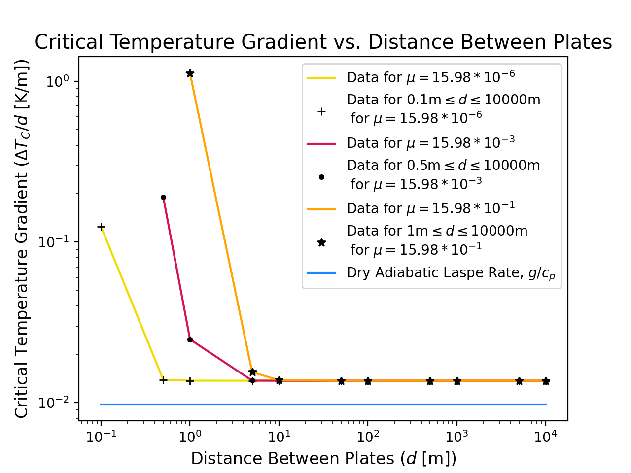

We found that the range of plate separation distance $d$ over which the Boussinesq assumption is applicable to the compressible case depends on the viscosity of the fluid. In particular, there is some clearly-defined viscosity-dependent value of $d$, which we have determined quantitatively, at which the compressible solution deviates from the Boussinesq solution. This value of $d$ is larger for a more viscous fluid. It is interesting that this deviation comes at scales as small as 1m, although it is not unexpected, based solely on the requirement that the imposed temperature gradient must overcome the adiabatic lapse rate. It should be noted that these results do not imply that the anelastic equations must be employed at all scales greater than 1m. In particular, in a stably stratified layer vertical motion is inhibited, and in the limit as $w$ goes to zero, we recover an incompressible fluid (see equation~\ref{eq:cont}), in which the effects of gravity are not important. Thus, it is only important to consider the anelastic equations in cases when there is significant vertical motion.

Another deviation between the compressible and Boussinesq cases occurs in the $a_c = 3.1/d$ relation at large plate separation distance $d$. For the lowest viscosity, the deviation is orders of magnitude for $d=10000$m; the corresponding horizontal wave length of the convection rolls in the compressible fluid is of the order of $1000$km. This result, however, must be taken with caution, as should all results at the largest plate separation distances, because the assumptions of our model are only valid when the plate separation is small relative to the scale height. For the parameters that we considered, this scale height is of the order of $7$km, which means that we cannot be sure of our results for the largest $d$ that we considered. In addition, we also observed larger changes in the computed values when performing the computations on a finer grid. It is for this reason that the two largest values of $d$ are not included in the calculation of the intersections for Fig. 3a and Fig. 4, so we can maintain confidence in the results of the change in the behaviour.

Near the onset of convection, the structure of the convective rolls can often be approximately determined by the eigenfunction (i.e. the perturbation) corresponding to the zero eigenvalue. Furthermore, because the eigenvalue is real, we would expect the flow to be steady. We do not prove these here, because the proof would have to take into consideration the nonlinear terms in the governing equations. Thus, the form of the convective rolls is determined by the value of the critical wave number $a_c$ for a given $d$, and the vertical part of the eigenfunction $U=[\hat{\psi}(z),\hat{T}(z)]$ (see Eq. \ref{eq:soln_form} and Eq. \ref{eq:eig_prob}). Fig. 3 shows a contour plot of an example of the temperature portion of the eigenfunction for $d=1000$m; the corresponding plots for all other plate separation distances $d$ have similar form. The real part of the eigenfunction is plotted; the imaginary part is the same, but with a shifted spatial phase. The horizontal structure of the rolls is periodic with period $2 \pi/a_c$, and the vertical structure is symmetric about the mid-plane, with a maximum occurring at the mid-plane. This follows with the expected straight, parallel convection rolls that occur near the onset of convection. (5, 6) The vertical cross section through height, which is not shown here, also matches what was found in Spiegel (1965). (12)

In this paper, we have studied the onset of convection in a compressible fluid contained between two infinite horizontal plates. We use a model that is inspired by the parameters found for the Earth's atmosphere. However, in order to simplify the analysis, we consider an isothermal atmosphere and we incorporate an assumption that restricts its applicability to plate separations that are less than the troposphere's height. These assumptions are sufficient to explore the region in which the solutions of the Boussinesq equations begin to differ from those of the anelastic equations. Future work will investigate the effects of relaxing these assumptions and will also include exploring the effects of a rotating system ($\vec{\Omega} \neq 0$) or one with internal sources of heat ($Q \neq 0$).

Acknowledgements

G.M. Lewis would like to acknowledge support from the Natural Sciences and Engineering Research Council of Canada (NSERC). The authors would also like to thank the reviewers for their comments, which provided insight to improve this work.

References

1. Rayleigh, L. 1916. “LIX. On convection currents in a horizontal layer of fluid, when the higher temperature is on the under side.” The London, Edinburgh, and Dublin Philosophical Magazine and Journal of Science 32 (192): 529–546. https://doi.org/10.1080/14786441608635602.
2. Chitre, S. M., and M. H. Gokhale. 1973. “Convective instability in a compressible atmosphere.” Solar Phys. 30:309–318. https://doi.org/10.1007/BF00152662.
3. Busse, F. H. 1978. “Non-linear properties of thermal convection.” Reports on Progress in Physics 41, no. 12 (December): 1929–1967. https://doi.org/10.1088/0034-4885/41/12/003. https://doi.org/10.1088/0034-4885/41/12/003.
4. Busse, F. H. 1989. Fundamentals of thermal convection. In Mantle Convection: Plate Tectonics and Global Dynamics, edited by W. Peltier. 23–95. Montreux: Gordon / Breach.
5. Bodenschatz, E., W. Pesch, and G. Ahlers. 2000. “Recent Developments in Rayleigh-Bénard Convection.” Annual Review of Fluid Mechanics 32(1): 709–778. https://doi.org/10.1146/annurev.fluid.32.1.709.
6. Schlüter, A., D. Lortz, and F. Busse. 1965. “On the stability of steady finite amplitude convection.” Journal of Fluid Mechanics 23 (1): 129–144. https://doi.org/10.1017/S0022112065001271.
7. Kurowski, M. J., W. W. Grabowski, and P. K. Smolarkiewicz. 2014. “Anelastic and Compressible Simulation of Moist Deep Convection.” Journal of the Atmospheric Sciences (Boston MA, USA) 71, no. 10 (October): 3767–3787. https://doi.org/10.1175/JAS-D-14-0017.1.
8. Lipps, F. B. 1990. “On the Anelastic Approximation for Deep Convection.” Journal of Atmospheric Sciences 47, no. 14 (July): 1794–1798. https://doi.org/10.1175/1520-0469(1990)047<1794:OTAAFD>2.0.CO;2.
9. Boussinesq, J. 1903. Théorie analytique de la chaleur. Vol. 2. Paris: Gauthier-Villars.
10. Spiegel, E. A., and G. Veronis. 1960. “On the Boussinesq Approximation for a Compressible Fluid.” Astrophysical Journal 131:442–447.
11. Jeffreys, H. 1930. “The Instability of a Compressible Fluid heated below.” Mathematical Proceedings of the Cambridge Philosophical Society 26 (2): 170–172. https://doi.org/10.1017/S0305004100015413.
12. Spiegel, E. A. 1965. “Convective Instability in a Compressible Atmosphere. I.” 141 (April): 1068–1090. https://doi.org/10.1086/148197.
13. Tilgner, A. 2011. “Convection in an ideal gas at high Rayleigh numbers.” Phys. Rev. E 84 (2): 026323. https://doi.org/10.1103/PhysRevE.84.026323.
14. Ogura, Y., and J. G. Charney. 1960. “A numerical model of thermal convection in the atmosphere.” Proc. Internat. Symposium on Numerical Weather Prediction, 431–452.
15. Gough, D. O. 1969. “The Anelastic Approximation for Thermal Convection.” Journal of Atmospheric Sciences (Boston MA, USA) 26, no. 3 (May): 448–456. https://doi.org/10.1175/1520-0469(1969)026<0448:TA-AFTC>2.0.CO;2.
16. Burnishev, Y., E. Segre, and V. Steinberg. 2010. “Strong symmetrical non-Oberbeck–Boussinesq turbulent convection and the role of compressibility.” Physics of Fluids 22 (3): 035108. https://doi.org/10.1063/1.3358462. https://doi.org/10.1063/1.3358462.
17. Robinson, F., and K. Chan. 2004. “Non-Boussinesq simulations of Rayleigh–Bénard convection in a perfect gas.” Physics of Fluids 16 (5):1321–1333. https://doi.org/10.1063/1.1689350. https://doi.org/10.1063/1.1689350.
18. Acheson, D. J. 1990. Elementary Fluid Dynamics. Oxford: Clarendon Press.
19. Kundu, P., and I. Cohen. 2002. Fluid Mechanics. 2nd ed. San Diego, CA: Academic Press.
20. Holton, J. R. 2004. An Introduction to Dynamic Meteorology. Burlington, MA: Elsevier Academic Press

Simzer & Lewis. MSURJ, 16, 1, 50-56 (2021)